## This Rmarkdown script uses the following libraries. You may need to run one of the two scripts
## #`install-packages.R` or `install-common-packages.R` first if these packages aren't already loaded into RStudio. ## (Both scripts do the same thing, but `install-packages.R` is written in a more elegant way.)

library(googlesheets4)
library(googledrive)
library(tidyr)
library(readr)
library(plyr) # should be invoked before dplyr
library(dplyr)
library(stringr)
library(reactable)
library(forcats)
library(ggplot2)
library(ggtext)
library(ggalluvial)
library(skimr)
library(stringr)
library(janitor) # for tabyl
library(flextable)
library(scales)
library(GGally)
library(webshot)
library(magick)
library(knitr)
library(kableExtra)
library(forcats)
library(ggfittext)
library(hrbrthemes)
library(janitor)Bolivia Studies Journal Data Page
This page is supplementary material to Carwil Bjork-James’s article, “Tactics of political violence in the 2019 Bolivian crisis: Return of the catastrophic stalemate?,” to be published in the Bolivian Studies Journal.
All queries and data tables referenced in the article are compiled in BSJ-Political-Violence.Rmd in the Ultimate Consequences package on GitHub, using the database as constituted on November 16, 2022. A copy of the database on that date is archived for reproducibility of the analysis as data/deaths-entries-2022-11-16.rds. Access is currently available to researchers on request and will be incorporated into the forthcoming public release of the dataset. The queries, data tables, and code used to create them are published online as Bjork-James 2022 at https://ultimateconsequences.github.io/BSJ-Political-Violence.html.
This document is designed to enable transparency and reproducibility of our research results. By specifying our search criteria for relevant cases, explaining exceptions, and embedding our analysis techniques in R scripts that use the database, we document our choices and create tools that can automatically update results when additional cases are uncovered, errors are corrected, or new information is brought to light. Archiving and versioning of the database and these tools allows other researchers to both reproduce our results, and test their robustness against different choices in coding or analysis.
This document is divided into two parts. Unless you are attempting to reproduce our results from the dataset, feel free to skip over Preparatory Code Blocks, and begin reading at Calculations and Queries Used in the Article.
For more information about the Ultimate Consequences research project, database, and future testimonial archive, head to our Project Overview page.
Preparatory Code Blocks
The following sections show all code in R needed to read and process the database. It is included here to allow researchers using R to reproduce the analysis from an archived copy of the dataset. Similarly, text below documents the standard importing, filtering, and processing of the data.
First, import the data from Google Sheets or retrieve it from the package
This code can either live-import the dataset from its Google Sheets instantiation or reload an already imported dataset stored in the GitHub package. The former will only run successfully if… - You have been granted access to the Google Sheet - You have the “Bolivia Deaths Database” in the root directory of your Google Drive. - You accept giving “Tidyverse API” access to your Google Drive.
Doing this is not needed for reproducibility of the results. Just keep the code as-is below and you will access the database as it was imported at the time of final article submision.
This code segment applies a set of standard filters:
Culling out currently inactive variables using
selectSegmenting out parenthetical annotations using
separate:Answer (explanation)is split into two separate variables, the first holding a categorical variable, and the second holding the corresponding notes.
We also import a basic table of presidential terms from the database.
live.import <- FALSE

de.filename <- "data/deaths-entries-2022-11-16.rds"
pt.filename <- "data/presidents-table-2022-11-16.rds"
use.current.archive <- FALSE # This flag should be set to true when
# the above filenames do not have a datelibrary(here)
source(here::here("src","01-import-de-pt.R"), local = knitr::knit_global())
source(here::here("src","data-cleaning.R"), local = knitr::knit_global())
de.imported <- de # keep a copy around for debugging
pt <- clean_pt_variables(pt)
# create a smaller presidents table just for the study period
studyperiod.start <- as.Date("1982-10-10")
studyperiod.end <- Sys.Date()
pt.study <- pt %>% filter((first_day >= studyperiod.start) & (last_day <= studyperiod.end))Next, process the variables
First, we want to think through which variables are involved. They are:
pres_admin— who was the president?protest_domain— The broad arena of politial conflict. Tells us whether to count something as a coca death, or an armed actor deathstate_perpetrator— Was this death perpetrated by the state?
These are standard blocks of code, which currently appear in Database Overview.Rmd, and eventually will find a home in a variable set-up function. What does this code do?
pres_admin— While imported as a text variable, we want to treat pres_admin as an ordered factor, since presidencies are arranged in chronological, not alphabetical order.president_levelsis a vector that puts them in order. We usemutateto recst the variablepres_adminas a factor with these ordered levels. The summary table produced bytabylshows them in order.protest_domain— Protest domain is an unordered factor, so it’s okay if we leave it as just a character variable. In fact, this helps us when we search for the word “coca” in the factor.state_perpetrator— State perpetrator is a quasilogical variable. The code below takes the all the available factor values and merges them in to a Yes/No/Disputed/Unknown rubric.
library(janitor) # for tabyl

## Factoring: Presidential administration

president_levels <- c(
  "Hernán Siles Zuazo", "Víctor Paz Estenssoro", "Jaime Paz Zamora",
  "Gonzalo Sanchez de Lozada (1st)", "Hugo Banzer (2nd)", "Jorge Quiroga",
  "Gonzalo Sanchez de Lozada (2nd)", "Carlos Diego Mesa Gisbert",
  "Eduardo Rodríguez", "Evo Morales", "Interim military government",
  "Jeanine Áñez", "Luis Arce") # All presidencies, in chronological order
president_initials <- c(
  "HSZ", "VPE", "JPZ",
  "GSL", "HB", "JQ",
  "GSL", "CM",
  "ER", "EM", "Mil",
  "JA", "LA")

de <- de %>% mutate(pres_admin=factor(pres_admin, levels=president_levels))
de %>% tabyl(pres_admin)  %>%
  adorn_totals("row") %>%
  adorn_pct_formatting()
pres_admin n percent
Hernán Siles Zuazo 8 1.2%
Víctor Paz Estenssoro 43 6.7%
Jaime Paz Zamora 21 3.3%
Gonzalo Sanchez de Lozada (1st) 51 7.9%
Hugo Banzer (2nd) 121 18.8%
Jorge Quiroga 33 5.1%
Gonzalo Sanchez de Lozada (2nd) 146 22.7%
Carlos Diego Mesa Gisbert 19 3.0%
Eduardo Rodríguez 0 0.0%
Evo Morales 148 23.0%
Interim military government 9 1.4%
Jeanine Áñez 26 4.0%
Luis Arce 19 3.0%
Total 644 100.0%## Factoring: State perpetrator (a quasilogical variable)
de %>% tabyl(state_perpetrator) %>%
adorn_totals("row") %>%
adorn_pct_formatting() state_perpetrator n percent valid_percent
Disputed 4 0.6% 0.6%
In mutiny 5 0.8% 0.8%
Indirect 15 2.3% 2.4%
Likely Yes 4 0.6% 0.6%
Likely no 3 0.5% 0.5%
No 286 44.4% 45.8%
Presumed Yes 7 1.1% 1.1%
Presumed yes 2 0.3% 0.3%
Unknown 1 0.2% 0.2%
Yes 298 46.3% 47.7%
<NA> 19 3.0% -
Total 644 100.0% 100.0%de$state_perpetrator <- fct_explicit_na(de$state_perpetrator, na_level = "Unknown")Warning: `fct_explicit_na()` was deprecated in forcats 1.0.0.
ℹ Please use `fct_na_value_to_level()` instead.de$state_perpetrator <- fct_collapse(de$state_perpetrator,
Yes = c("Yes", "Likely Yes", "Presumed Yes", "Presumed yes"),
Indirect = c("Indirect"),
No = c("No", "Likely no"),
Mutiny = c("In mutiny"),
Unknown = c("Unknown", "Disputed", "Suspected") )Warning: Unknown levels in `f`: Suspectedde$state_perpetrator <- fct_relevel(de$state_perpetrator,
c("Unknown", "No", "Indirect", "Mutiny", "Yes"))
de %>% tabyl(state_perpetrator) %>%
adorn_totals("row") %>%
adorn_pct_formatting() state_perpetrator n percent
Unknown 24 3.7%
No 289 44.9%
Indirect 15 2.3%
Mutiny 5 0.8%
Yes 311 48.3%
Total 644 100.0%## Factoring: State perpetrator (a categorical variable)
de.imported %>% tabyl(state_responsibility) %>%
adorn_totals("row") %>%
adorn_pct_formatting() # Look at it before state_responsibility n percent valid_percent
Political victim 2 0.3% 0.3%
Political victim / political perpetrator 1 0.2% 0.2%
Political victim / unknown perpetrator 3 0.5% 0.5%
Separate from state 197 30.6% 31.6%
Seperate from state 1 0.2% 0.2%
State indirect perpetrator 3 0.5% 0.5%
State involved 46 7.1% 7.4%
State likely perpetrator 5 0.8% 0.8%
State perpetrator 291 45.2% 46.6%
State perpetrator, State victim in mutiny 9 1.4% 1.4%
State perpetrator, State victim refusing orders 1 0.2% 0.2%
State victim 60 9.3% 9.6%
State victim, State perpetrator in mutiny 5 0.8% 0.8%
<NA> 20 3.1% -
Total 644 100.0% 100.0%# This code lets us look ta relevant cases of unintential death
#
# de %>% filter((intentionality=="Conflict Accident")|(intentionality=="Nonconflict Accident")|
# (intentionality=="Incidental")) -> de.acc
#
# de.acc %>% tabyl(state_responsibility)
# de.acc %>% filter(state_responsibility=="Victim")
de <- de %>% mutate(state_responsibility = case_when( # overwrite the state responsibility for unintentional cases
intentionality == "Incidental" ~ "Incidental",
intentionality == "Conflict Accident" ~ "Accidental",
TRUE ~ state_responsibility))
de$state_responsibility <- fct_explicit_na(de$state_responsibility, na_level = "Unknown")
de$state_responsibility <- fct_collapse(de$state_responsibility,
Perpetrator = c("State perpetrator", "State likely perpetrator",
"State perpetrator, State victim refusing orders",
"State perpetrator, State victim in mutiny",
"State indirect perpetrator"),
Involved = c("State involved", "Political victim",
"Political victim / political perpetrator",
"Political victim / unknown perpetrator",
"Possibly state involved"),
Victim = c("State victim",
"State victim, State perpetrator in mutiny"),
Separate = c("Separate from state"),
Unintentional = c("Incidental", "Accidental"),
Unknown = c("Unknown", "Unclear") )Warning: Unknown levels in `f`: Possibly state involved, Unclearsr_levels <- c("Perpetrator", "Victim", "Involved", "Separate", "Unintentional", "Unknown")
de$state_responsibility <- fct_relevel(de$state_responsibility, sr_levels)
state_resp.colors <- c(
Perpetrator = "forestgreen",
Victim = "firebrick4",
Involved = "lightgreen",
Separate = "goldenrod2",
Unintentional = "darkgray",
Unknown = "lightgray")
de %>% tabyl(state_responsibility) %>%
adorn_totals("row") %>%
adorn_pct_formatting() # Look at it after state_responsibility n percent
Perpetrator 307 47.7%
Victim 63 9.8%
Involved 28 4.3%
Separate 191 29.7%
Unintentional 36 5.6%
Unknown 18 2.8%
Seperate from state 1 0.2%
Total 644 100.0%Note that this leaves us with two variables for understanding the state’s role.
The simplified
state_perpetratorvariable is a factor with four levels: Yes, Mutiny, Indirect, No, and UnknownThe simplified
state_responsibilityvariable is more concerned in sorting out whether the state was present as victim or perpetrator, was involved in the dispute, or it was separate from the state.
The “standard filters” on the dataset remove the following cases:
unconfirmedis a flag for deaths in range of death totals. So if there were “five to eight people killed,” the last three deaths have TRUE inunconfirmed.We also filter out “Collateral”, “Nonconflict”, and “Nonconflict Accident” cases in
Intentionality. These cases are both peripheral to some of the purposes of the database. Significantly for comparisons over the long-term, we think that these kinds of deaths are unevenly distributed over time.
def <- de %>%
  filter(is.na(unconfirmed) | unconfirmed != TRUE) %>%
  filter(is.na(intentionality) | intentionality != "Collateral") %>%
  filter(is.na(intentionality) | intentionality != "Nonconflict Accident") %>%
  filter(is.na(intentionality) | intentionality != "Nonconflict")

de.confirmed <- def
Function to generate a summary data table based on on variable
## Make a generic function to summarize deaths according to the columns
## in our Categorized Deaths table
n_categorized_by <- function(de, by, complete = FALSE){
  output <- de %>%
    filter(!is.na({{by}})) %>%
    filter({{by}} != "") %>%
    group_by( {{ by }} ) %>%
    dplyr::summarize(
      n = n(), # all deaths
      n_coca = sum(str_detect(protest_domain, "Coca"), na.rm = TRUE), #coca deaths
      n_armedactor =sum((protest_domain=="Guerrilla") |
                          ( protest_domain == "Paramilitary"),
                        na.rm = TRUE), # armed actor death
      n_state_perp = sum(state_perpetrator=="Yes", na.rm = TRUE), #state perp
      n_state_perp_coca = sum(((state_perpetrator=="Yes") & (str_detect(protest_domain, "Coca"))), na.rm = TRUE), #state perp coca death
      n_state_perp_armedactor = sum((state_perpetrator=="Yes" & ((protest_domain=="Guerrilla") | ( protest_domain == "Paramilitary" ))), na.rm = TRUE), #state perp armed actor death,
      n_state_perp_ordinary = n_state_perp - n_state_perp_armedactor - n_state_perp_coca, # all other state perp deaths
      n_state_victim = sum(state_responsibility=="Victim", na.rm = TRUE), # state victim
      n_state_victim_coca = sum(((state_responsibility=="Victim") &
                                   (str_detect(protest_domain, "Coca"))), na.rm = TRUE), #state victim coca death
      n_state_victim_armedactor = sum(((state_responsibility=="Victim") &
                                         ((protest_domain=="Guerrilla") |
                                            (protest_domain == "Paramilitary"))), na.rm = TRUE), #state victim armed actor death
      n_state_victim_ordinary = n_state_victim - n_state_victim_armedactor - n_state_victim_coca, # all other state perp deaths
      n_state_separate = sum(str_detect(state_responsibility, "Separate"), na.rm = TRUE),
      n_remaining = n - n_state_perp - n_state_victim,
      n_remaining_coca = n_coca - n_state_perp_coca - n_state_victim_coca,
      n_remaining_armedactor = n_armedactor - n_state_perp_armedactor - n_state_victim_armedactor
    )

  if(complete){
    output <- output %>%
      complete({{by}}, fill =list(
        n = 0,
      n_coca = 0,
      n_armedactor = 0,
      n_state_perp = 0,
      n_state_perp_coca = 0,
      n_state_perp_armedactor = 0,
      n_state_perp_ordinary = 0,
      n_state_victim = 0,
      n_state_victim_coca = 0,
      n_state_victim_armedactor = 0,
      n_state_perp_ordinary = 0,
      n_state_separate = 0,
      n_remaining = 0,
      n_remaining_coca = 0,
      n_remaining_armedactor = 0
      ))
  }

  return(output)
}
Calculations and Queries Used in the Article
Deadliest events
Thirty-eight lives were lost during the crisis, a toll only exceeded by the September–October 2003 Gas War (with 70 deaths), though closely followed by the February 2003 tarifazo tax protests (35 deaths).
de.confirmed %>% tabyl(event_title) %>% filter(n>20) %>% select(-percent) %>% arrange(desc(n)) event_title n
2003 Gas War 70
Tarifazo tax protest 35
Laymi-Qaqachaka 2000 29
Plan Dignity 1998 23An overall breakdown
n_entries <- nrow(de)
n_confirmed <- nrow(def)

n_unconfirmed <- sum(de$unconfirmed == TRUE, na.rm =TRUE)

de_excluded <- de %>%
  filter(intentionality == "Collateral"
         | intentionality == "Nonconflict Accident"
         | intentionality == "Nonconflict")
n_excluded <- nrow(de_excluded)
n_collateral <- sum(de$intentionality == "Collateral", na.rm = TRUE)
n_nonconfaccident <- sum(de$intentionality == "Nonconflict Accident", na.rm = TRUE)
n_nonconfdeath <- sum(de$intentionality == "Nonconflict", na.rm = TRUE)

de_named <- de %>%
  filter(!is.na(dec_firstname) & !is.na(dec_surnames) )
n_named <- nrow(de_named)
The database includes 626 to 644 of these deaths, including those of 595 named individuals.
Note: Of the 644 deaths recorded in the database, 18 are “unconfirmed” deaths corresponding to cases where an uncertain number of people were killed (e.g., if “three to five” people were reported killed, two unnamed individuals are included in the database as unconfirmed deaths). There are 13 recorded instances of non-conflict-related accidents and 3 non-conflict-related natural deaths associated with protest events; and 5 recorded instances of deaths from medical causes, where protest or repression may have impeded medical care (“collateral”). For the remainder of this article, we refer to the 605 deaths not excluded for any of these reasons as “confirmed deaths.”
Partisan Deaths
From 1982 until 2006, there were no deadly partisan street clashes in Bolivia, but they emerged dramatically during the stalemate.
Note that the 2001 Santa Rosa Massacre was not a street clash, but did target its victims by partisan affiliation.
de.confirmed %>% filter(protest_domain=="Partisan Politics") %>%
                 filter(pol_assassination=="No") %>%
                 select(event_title, year, dec_firstname, dec_surnames, cause_death, intentionality)
# A tibble: 63 × 6
event_title year dec_firstname dec_surnames cause_death intentionality
<chr> <int> <chr> <chr> <chr> <chr>
1 Santa Rosa Massacre 2001 Sandra Vásquez Gunshot Direct
2 Santa Rosa Massacre 2001 Ernesto Vásquez Mosqueira Gunshot Direct
3 Santa Rosa Massacre 2001 Ernesto Vásquez Gunshot Direct
4 Santa Rosa Massacre 2001 Esmir Vásquez Mosqueira Gunshot Direct
5 11 de Enero clashes 2007 Christian Urresti Strangled Direct
6 11 de Enero clashes 2007 Juan Ticacolque Machaca Gunshot Direct
7 11 de Enero clashes 2007 Luciano Colque Beating Direct
8 Sucre constitution protest 2007 Gonzalo Durán Carazani Gunshot Direct
9 Sucre constitution protest 2007 José Luis Luis Cardozo Lazcano Gunshot Direct
10 Sucre constitution protest 2007 Juan Carlos Serrado Murillo Impact Direct
# ℹ 53 more rowsArson Deaths
During the past four decades, there were only two deadly protest arsons in Bolivia: two Qaqachaka residents were killed when their home was burned in 1996; and a fire set by a protesting parents’ group at the El Alto City Hall in 2016 caused the deaths of five municipal workers.
de.confirmed %>% filter(cause_death=="Fire") %>%
                 select(event_title, year, dec_firstname, dec_surnames, cause_death, intentionality)
# A tibble: 13 × 6
event_title year dec_firstname dec_surnames cause_death intentionality
<chr> <int> <chr> <chr> <chr> <chr>
1 Laymi-Qaqachaka 1996 1996 <NA> <NA> Fire Direct
2 Laymi-Qaqachaka 1996 1996 <NA> <NA> Fire Direct
3 2003 Gas War 2003 Braulio Callisaya Dorado (Callizaya) Fire Conflict Accident
4 2003 Gas War 2003 Raul Flores Huanca Fire Conflict Accident
5 2003 Gas War 2003 Florentino Poma Flores Fire Conflict Accident
6 2003 Gas War 2003 Benita Rodriguez (Rodriguez Ticona) Fire Conflict Accident
7 2003 Gas War 2003 Dominga Rodriguez (Rodriguez de Tapia) Fire Conflict Accident
8 Santa Cruz loteadores clash 2010 Marco Antonio Gómez Carrasco Fire Direct
9 El Alto City Hall protest arson 2016 Ana María Apaza Alanoca Fire Direct
10 El Alto City Hall protest arson 2016 Javier Mollericona Quispe Fire Direct
11 El Alto City Hall protest arson 2016 José Rodrigo Cortez Flores Fire Direct
12 El Alto City Hall protest arson 2016 Rosmery Mamani Paucara Fire Direct
13 El Alto City Hall protest arson 2016 Gloria Magaly Calle Suarez Fire Direct de.confirmed %>% filter(weapon=="Arson") %>%
select(event_title, year, dec_firstname, dec_surnames, cause_death, intentionality)# A tibble: 7 × 6
event_title year dec_firstname dec_surnames cause_death intentionality
<chr> <int> <chr> <chr> <chr> <chr>
1 Laymi-Qaqachaka 1996 1996 <NA> <NA> Fire Direct
2 Laymi-Qaqachaka 1996 1996 <NA> <NA> Fire Direct
3 El Alto City Hall protest arson 2016 Ana María Apaza Alanoca Fire Direct
4 El Alto City Hall protest arson 2016 Javier Mollericona Quispe Fire Direct
5 El Alto City Hall protest arson 2016 José Rodrigo Cortez Flores Fire Direct
6 El Alto City Hall protest arson 2016 Rosmery Mamani Paucara Fire Direct
7 El Alto City Hall protest arson 2016 Gloria Magaly Calle Suarez Fire Direct A sixth worker was beaten to death. In addition, police fatally shot a protesting university student during the attempted destruction of the Transit Police building in Sucre on November 25, 2007, and policeman Juan Alcón Parra was fatally beaten as protesters took over and ultimately burned the Regional Police Command in El Alto on November 11, 2019.
Descriptions retrieved from the database narratives.
Security Force Shootings
de.spgunshot <- de.confirmed %>% filter(cause_death=="Gunshot" & state_perpetrator == "Yes") %>%
                 select(event_title, year, dec_firstname, dec_surnames, cause_death, intentionality,
                        perp_category)

de.spgunshot.table <- de.spgunshot %>% tabyl(event_title) %>% filter(n>=3) %>%
                                       select(-percent) %>% arrange(desc(n))

de.spgunshot.table
event_title n
2003 Gas War 53
Tarifazo tax protest 28
Senkata Massacre 11
Sacaba massacre 10
CSUTCB mobilization September 2000 8
Chayanta mining strike 8
Jan 2003 coca clashes 7
Plan Dignity 1998 7
Chapare cocalero protests 2001 6
Eterazama eradication 5
Sacaba-Chapare coca market conflict 5
Villa Tunari Massacre 5
Cooperative miner strike 4
Isinuta DEA confrontation 4
La Paz raid on CNPZ 4
Santa Ana de Yacuma drug trafficking raid 4
CSUTCB mobilization April 2000 3
Coca eradication 1995 3
La Paz post-resignation violence 3
Pensioner strike 3
Santa Cruz raid on Rosza group 3n_spgunshot.events <- nrow(de.spgunshot.table)
n_spgushot.bystanders <- de.confirmed %>% filter((cause_death=="Gunshot" & state_perpetrator == "Yes")&
(intentionality=="Bystander")) %>%
nrow()
n_spgushot.bystanders_hi <- de.confirmed %>% filter((cause_death=="Gunshot" & state_perpetrator == "Yes")&
(intentionality=="Bystander" |
intentionality == "Direct / Bystander")) %>%
nrow()There have been at least 21 events in which security forces shot three or more people during protests, and 28 to 43 times that security forces killed bystanders, often by firing indiscriminately beyond those protesting.
Deadliest events and Gas War summary
The Sacaba and Senkata massacres were the deadliest episodes of state violence since the 2003 Gas War, when the security forces killed 59 people over four weeks. Forty-eight of them died the weekend of October 11–13, 2003, when a militarized convoy ran another blockade at Senkata.
This code first creates a table of all events with at least 10 state-perpetrated deaths, sorted chronologically by year and month. Next it creates a table of Gas War deaths, counts them, and provides a list by date of deadly incident.
events.table <- def %>% group_by(event_title, year, month) %>%
  dplyr::summarize(
    n = n(),
    n_state_perp = sum(state_perpetrator=="Yes", na.rm = TRUE),
    n_state_victim = sum(state_responsibility=="State victim", na.rm = TRUE),
    n_state_separate = sum(str_detect(state_responsibility, "Separate from state"), na.rm = TRUE)
  )
`summarise()` has grouped output by 'event_title', 'year'. You can override using the `.groups` argument.events.table %>% filter(n_state_perp>=10) %>% arrange(year, month)# A tibble: 7 × 7
# Groups: event_title, year [7]
event_title year month n n_state_perp n_state_victim n_state_separate
<chr> <int> <int> <int> <int> <int> <int>
1 Villa Tunari Massacre 1988 6 10 10 0 0
2 Chayanta mining strike 1996 12 11 10 0 0
3 Plan Dignity 1998 1998 4 12 11 0 0
4 Tarifazo tax protest 2003 2 35 29 0 0
5 2003 Gas War 2003 10 65 55 0 0
6 Sacaba massacre 2019 11 10 10 0 0
7 Senkata Massacre 2019 11 11 11 0 0## Gas War calculations
def.gaswar.sp <- def %>% filter(protest_campaign=="2003 Gas War") %>%
filter(state_perpetrator=="Yes") # table of state perpetrator deaths in the 2003 Gas War
n_gaswar.sp <- nrow(def.gaswar.sp) # count them
def.gaswar.sp %>% select(year, month, day, dec_firstname, dec_surnames) #output a table with dates and names# A tibble: 59 × 5
year month day dec_firstname dec_surnames
<int> <int> <int> <chr> <chr>
1 2003 9 20 Demetrio (Primitivo) Coraca Castro
2 2003 9 20 Juan Cosme Apaza
3 2003 9 20 Simael Marcos (Ismael, Gilmer Marcos) Quispe Quispe (Quispe Apaza)
4 2003 9 20 Marlene Nancy Rojas Ramos
5 2003 10 9 José Luis Atahuichi Ramos
6 2003 10 9 Ramiro Vargas Astilla
7 2003 10 11 Walter Huanca Choque
8 2003 10 11 Alex Llusco Mollericona
9 2003 10 11 Raul Marca Ruiz
10 2003 10 11 José Miguel Pérez Cortez
# ℹ 49 more rowsTable 3
Overall conflict deaths declined sharply as well, though not quite to the levels that had reigned prior to 2000. The Morales years did see repeated episodes of violence between civilian groups: partisans and those in local disputes over mines and land. The first three weeks of the 2019 crisis continued this trend. Table 3
This statement about repression relies on dividing time up into five periods. (Rather than drawing a conclusion about the brief and ongoing Arce government, I leave it off the table in the article.)
presidents.calm=str_c("Carlos Diego Mesa Gisbert", "Eduardo Rodríguez", "Evo Morales", sep = "|")
presidents.righti=str_c("Interim military government", "Jeanine Áñez", sep = "|")

def.periods <- def %>% mutate(period = case_when(
  year < 2000 ~ "A. Oct 1982–1999",
  (year>=2000)&(year<2003) ~ "B. 2000–2003",
  (year == 2003) & (str_detect(string = pres_admin, pattern="Gonzalo Sanchez de Lozada \\(2nd\\)"))~ "B. 2000–2003",
  str_detect(string = pres_admin, pattern=presidents.calm) ~ "C. 2004–Nov 2019",
  str_detect(string = pres_admin, pattern=presidents.righti) ~ "D. Nov 2019–Nov 2020",
  (pres_admin=="Luis Arce") ~ "E. Nov 2020-present",
  TRUE ~ ""))

def.periods %>% select(event_title, year, period) -> defpcheck # simplify to make sure it worked

repression.periods.categorized <- def.periods %>%
  n_categorized_by(period, complete=TRUE) %>%
  select(period, n, n_state_perp) %>%
  mutate(perc_state_perp = percent(n_state_perp / n, accuracy = 1) )

repression.periods.categorized <-
  repression.periods.categorized %>% mutate(days=c(
           -as.numeric(difftime("1982-10-10", "2000-01-01", units = "days")),
           -as.numeric(difftime("2000-01-01", "2003-10-19", units = "days")),
           -as.numeric(difftime("2003-10-19", "2019-11-10", units = "days")),
           -as.numeric(difftime("2019-11-10", "2020-11-08", units = "days")),
           -as.numeric(difftime("2020-11-08", "2022-11-16", units = "days"))), .after=period)

repression.periods.categorized <-
  repression.periods.categorized %>%
  mutate(years=days/365, .after=days) %>%
  mutate(n_peryear=n/years, .after=n)  %>%
  mutate(sp_peryear=n_state_perp/years, .after=n_state_perp)

repression.periods.categorized
# A tibble: 5 × 8
period days years n n_peryear n_state_perp sp_peryear perc_state_perp
<chr> <dbl> <dbl> <int> <dbl> <int> <dbl> <chr>
1 A. Oct 1982–1999 6292. 17.2 155 8.99 97 5.63 63%
2 B. 2000–2003 1387. 3.80 245 64.5 138 36.3 56%
3 C. 2004–Nov 2019 5866. 16.1 154 9.58 40 2.49 26%
4 D. Nov 2019–Nov 2020 364 0.997 34 34.1 30 30.1 88%
5 E. Nov 2020-present 738 2.02 17 8.41 0 0 0% Figure 1
plot <- def %>% filter(!is.na(protest_domain)) %>%
  ggplot(aes(x= year, fill = forcats::fct_rev(state_responsibility))) +
  geom_bar() +
  scale_fill_manual(limits = sr_levels, values = state_resp.colors, guide = guide_legend(reverse=TRUE)) +
  ggtitle("Conflict deaths by year and state responsibility, 1982-2022") +
  labs(fill = "State responsibility", y= "Number of deaths", x="Year") +
    theme(text=element_text(family="Alegreya Sans"),
          legend.position="right", legend.direction="vertical",  legend.key.height = unit(0.6, "lines"),
          legend.key.width=unit(2, "lines"),
          legend.text=element_text(size=11),
          axis.text=element_text(size=14),
          axis.title=element_text(size=10,face="bold"))


plot <- plot +
  annotate("rect", xmin = 1981.5,xmax = 1985.5,ymin = 0, ymax = Inf,
           fill="lightblue",
           alpha = .15)+
  annotate("text", x = 1983.5, y = 100, label = "bold(UDP)",
           parse = TRUE) +
  annotate("rect", xmin = 1985.5,xmax = 2005.5,ymin = 0, ymax = Inf,
              fill="darkgreen",
              alpha = .15)+
  annotate("text", x = 1995.5, y = 100, label = "bold(Neoliberal)",
           parse = TRUE) +
  annotate("rect", xmin = 2005.5,xmax = 2019,ymin = 0, ymax = Inf,
             fill="navyblue",
             alpha = .15) +
  annotate("text", x = 2012, y = 100, label = "bold(MAS-IPSP)",
           parse = TRUE) +
  annotate("rect", xmin = 2019,xmax = 2020,ymin = 0, ymax = Inf,
           fill="red",
           alpha = .15)+
  annotate("text", x = 2019.5, y = 100, label = "bold(Interim)",
           parse = TRUE) +
  annotate("rect", xmin = 2020,xmax = 2022.5,ymin = 0, ymax = Inf,
           fill="navyblue",
           alpha = .15)

plot
Warning: Removed 1 rows containing non-finite values (`stat_count()`).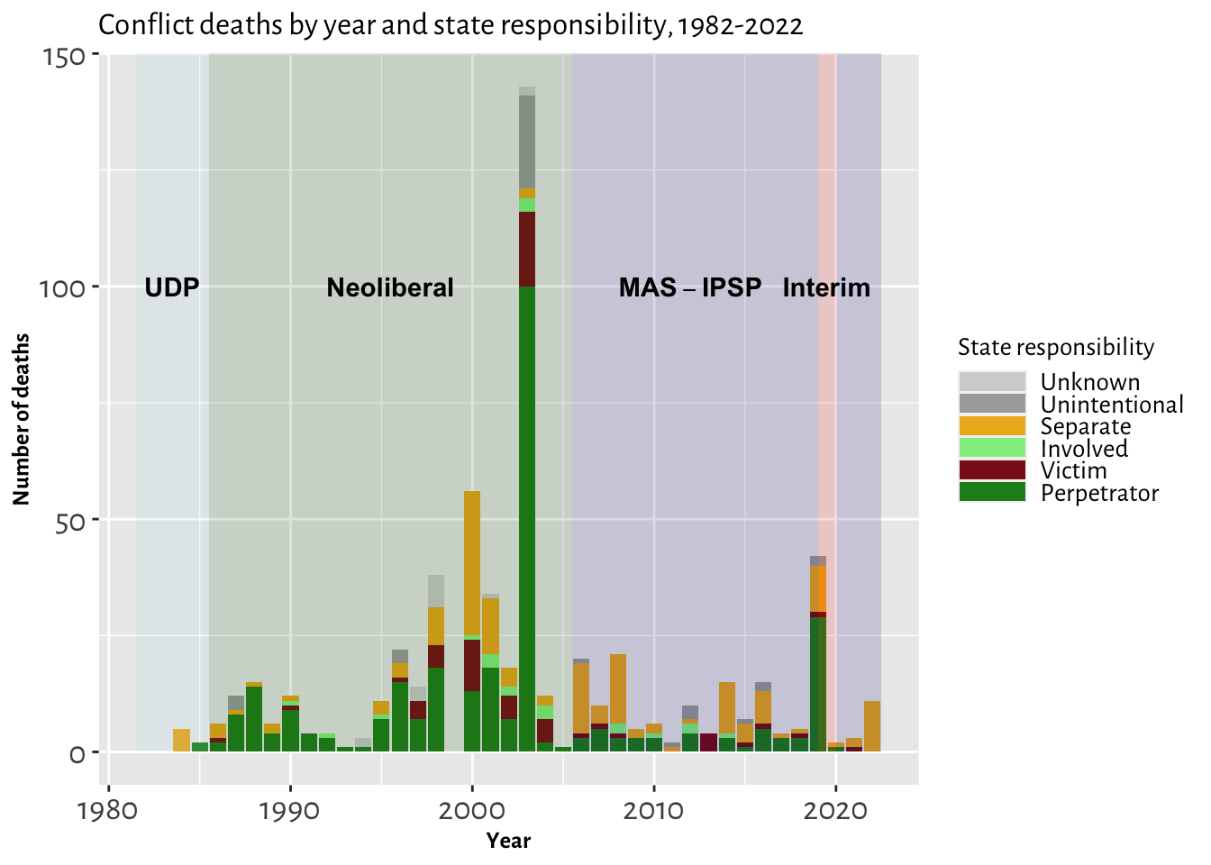
Background shading indicate political orientation of the government. The split background in 2019 and 2020 indicates that some deaths occurred under two different governments. However, all of the state perpetrator deaths in 2019 occurred during interim rule by the military or Jeanine Áñez. No interim shading appears in 2005 because all 2005 deaths were under Carlos Mesa. Entries: data/deaths-entries-2022-11-16.rds
Number of deaths by month
Thirty-eight people were killed (or fatally wounded) in the thirty-one days from the October 20 election to the Senkata massacre on November 19, making this the third-deadliest month in Bolivian political conflict since the October 1982 restoration of electoral democracy.
In terms of calendar months, only October 2003 and February 2003 had more deaths. In terms of a 31-day period, there are two distinct deadlier periods in January-February 2003 and September-October 2003.
library(reactable)
library(reactablefmtr)
Attaching package: 'reactablefmtr'The following object is masked from 'package:flextable':
voidThe following object is masked from 'package:ggplot2':
margin# First create a year/month table
def_valid_dates <- def %>%
filter(!is.na(year) & !is.na(month))
calendar_tibble <- def_valid_dates %>%
group_by(year, month) %>%
dplyr::summarize(N = n()) %>%
ungroup() %>%
complete(year = 1983:2022, month = 1:12,
fill = list(N = 0)) %>%
spread(month, N)`summarise()` has grouped output by 'year'. You can override using the `.groups` argument.calendar_tibble <- calendar_tibble %>% mutate(total = rowSums(.[2:13]))
names(calendar_tibble) <- c("Year", month.abb, "Total") # Add 3-char month names (in English)
calendar_tibble %>%
reactable(
theme = nytimes(),
defaultPageSize=25,
pageSizeOptions = c(10, 25, 40),
showPageSizeOptions=TRUE,
defaultColDef = colDef(
filterable=FALSE,
defaultSortOrder = "desc",
style = color_scales(calendar_tibble, span=2:13,
colors = c("#ffffff", "#ff3030")),
minWidth = 40, maxWidth=60),
)Entries: data/deaths-entries-2022-11-16.rds
State-perpetrator deaths by month
Altogether, thirty deaths were perpetrated by security forces, six during the interim military government and twenty-four under Jeanine Áñez. This remarkable toll exceeds the number of state-perpetrator deaths during the previous ten years, or the annual total of each year since 1982 except 2003.
In ten days, the police and military killed more protesters than they had in the previous ten years (22).
Annual totals are shown to the right of this monthly table of state-perpetrator deaths.
# First create a year/month table
def.sp_valid_dates <- def %>%
                  filter(state_perpetrator=="Yes") %>%
                  filter(!is.na(year) & !is.na(month))

calendar_tibble <- def.sp_valid_dates %>%
    group_by(year, month) %>%
    summarize(N = n()) %>%
    ungroup() %>%
    complete(year = 1983:2022, month = 1:12,
             fill = list(N = 0)) %>%
    spread(month, N)
`summarise()` has grouped output by 'year'. You can override using the `.groups` argument.calendar_tibble <- calendar_tibble %>% mutate(total = rowSums(.[2:13]))
names(calendar_tibble) <- c("Year", month.abb, "Total") # Add 3-char month names (in English)
calendar_tibble %>%
reactable(
theme = nytimes(),
defaultPageSize=25,
pageSizeOptions = c(10, 25, 40),
showPageSizeOptions=TRUE,
defaultColDef = colDef(
filterable=FALSE,
defaultSortOrder = "desc",
style = color_scales(calendar_tibble, span=2:13,
colors = c("#ffffff", "#ff3030")),
minWidth = 40, maxWidth=60),
)Entries: data/deaths-entries-2022-11-16.rds
de.sp.evo <- de.confirmed %>% filter(pres_admin=="Evo Morales" & state_perpetrator == "Yes")

n_sp_tenyears <- de.confirmed %>% filter((pres_admin=="Evo Morales" & state_perpetrator == "Yes") &
                                                  (year>2009) & (year<=2019)) %>%
                                          nrow()
as.numeric(n_sp_tenyears)
[1] 22About this R Markdown document
This is an R Markdown document. Markdown is a simple formatting syntax for authoring HTML, PDF, and MS Word documents. It allows for embedding R code inside a document. For more details on using R Markdown see http://rmarkdown.rstudio.com.
When you click the Knit button a document will be generated that includes both content as well as the output of any embedded R code chunks within the document. You can embed an R code chunk like this. (Note that the echo = FALSE parameter was added to the code chunk to prevent printing of the R code that generated the plot.)
# Why include this?
# See http://adv-r.had.co.nz/Reproducibility.html

sessionInfo()
R version 4.3.2 (2023-10-31)
Platform: aarch64-apple-darwin20 (64-bit)
Running under: macOS Ventura 13.6.7
Matrix products: default
BLAS: /Library/Frameworks/R.framework/Versions/4.3-arm64/Resources/lib/libRblas.0.dylib
LAPACK: /Library/Frameworks/R.framework/Versions/4.3-arm64/Resources/lib/libRlapack.dylib; LAPACK version 3.11.0
locale:
[1] en_US.UTF-8/en_US.UTF-8/en_US.UTF-8/C/en_US.UTF-8/en_US.UTF-8
time zone: America/Chicago
tzcode source: internal
attached base packages:
[1] stats graphics grDevices utils datasets methods base
other attached packages:
[1] reactablefmtr_2.0.0 here_1.0.1 hrbrthemes_0.8.0 ggfittext_0.10.2 kableExtra_1.4.0 knitr_1.45 magick_2.8.3 webshot_0.5.5 GGally_2.2.1 scales_1.3.0 flextable_0.9.4 janitor_2.2.0 skimr_2.1.5 ggalluvial_0.12.5 ggtext_0.1.2 ggplot2_3.4.4 forcats_1.0.0 reactable_0.4.4 stringr_1.5.1 dplyr_1.1.4 plyr_1.8.9 readr_2.1.5 tidyr_1.3.1 googledrive_2.1.1 googlesheets4_1.1.1
loaded via a namespace (and not attached):
[1] rlang_1.1.3 magrittr_2.0.3 snakecase_0.11.1 compiler_4.3.2 systemfonts_1.0.5 vctrs_0.6.5 httpcode_0.3.0 pkgconfig_2.0.3 crayon_1.5.2 fastmap_1.1.1 ellipsis_0.3.2 labeling_0.4.3 utf8_1.2.4 promises_1.2.1 rmarkdown_2.25 tzdb_0.4.0 ragg_1.2.7 purrr_1.0.2 xfun_0.42 jsonlite_1.8.8 later_1.3.2 uuid_1.2-0 R6_2.5.1 stringi_1.8.3 RColorBrewer_1.1-3 extrafontdb_1.0 lubridate_1.9.3 cellranger_1.1.0 Rcpp_1.0.12
[30] base64enc_0.1-3 extrafont_0.19 httpuv_1.6.14 timechange_0.3.0 tidyselect_1.2.0 rstudioapi_0.15.0 yaml_2.3.8 curl_5.2.0 tibble_3.2.1 shiny_1.8.0 withr_3.0.0 askpass_1.2.0 evaluate_0.23 ggstats_0.5.1 zip_2.3.1 xml2_1.3.6 pillar_1.9.0 generics_0.1.3 rprojroot_2.0.4 hms_1.1.3 munsell_0.5.0 xtable_1.8-4 glue_1.7.0 gdtools_0.3.5 tools_4.3.2 gfonts_0.2.0 data.table_1.15.0 fs_1.6.3 grid_4.3.2
[59] crosstalk_1.2.1 Rttf2pt1_1.3.12 colorspace_2.1-0 repr_1.1.6 cli_3.6.2 textshaping_0.3.7 officer_0.6.4 fontBitstreamVera_0.1.1 fansi_1.0.6 gargle_1.5.2 viridisLite_0.4.2 svglite_2.1.3 gtable_0.3.4 reactR_0.5.0 sass_0.4.8 digest_0.6.34 fontquiver_0.2.1 crul_1.4.0 farver_2.1.1 htmlwidgets_1.6.4 htmltools_0.5.7 lifecycle_1.0.4 mime_0.12 fontLiberation_0.1.0 gridtext_0.1.5 openssl_2.1.1